Understanding and Creating your own Classification Loss Function
In this blog, I firstly try to explain the classification loss function under geometrical perspective. Multiple loss functions will be tested with the Oxford-IIIT Pet Dataset using fastaiv2. The most simple loss function - dot product - will be introduced first, then we will try to create our own loss function to beat the most popular one - cross entropy loss function


Last week, I suddenly thought about Cross-Entropy loss function (the most popular loss function chosen for classification problem) while following fastai 2020 course. Actually I read about the proof of the function one or two times before and can understand it mathematically. However, I can not explain it naturally, and for me, naturally means there must have some images appear in my head when I think about it. The explanation should be natural, using normal language without using so much advanced math.
I then tried to review the topic, searched on the Internet for several resources, found some popular explanations with cross-entropy, probabilities or maximum likelihood which I was too lazy to read to the end. However, at this short article (https://medium.com/data-science-bootcamp/understand-cross-entropy-loss-in-minutes-9fb263caee9a), it has a part using dot-product to compare 2 vectors that shed a light to me.
The SoftMax final layer make the output likely be a probability distribution (its sum is 1), but it doesn't have to be thought in this way (even the Softmax layer is not obligatory). After all, it is a vector, and all we need is to predict a vector that is as close as possible to the target vector (for me, geometry is easier to imagine than probability)
We start firtly about what is a vector. A vector is just an arrow with a direction and length. So for the binary classification problem, we have an output vector which has 2 elements and sum up to 1. [p1, p2] and p1+p2 = 1
Imagine we want our target vector is [0,1]. The worst prediction is [0,1] and a good predition could be [0.99,0.01]
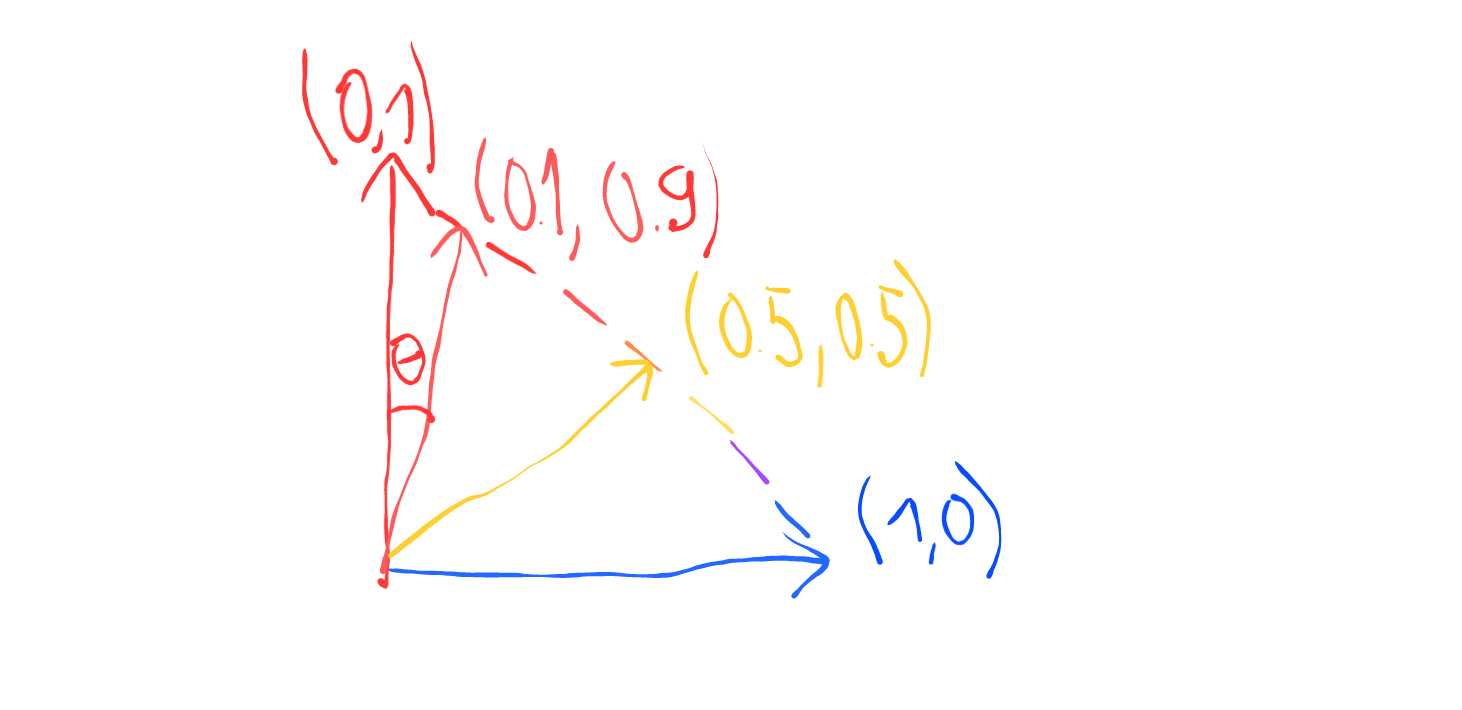
We notice that $cos(\theta)$ for $\theta$ from 0° to 90° decrese strictly from 1 to 0 (from the best to worst prediction) so it might be a good indicator for our prediction (And actually it exists, you can check for cosine similarity). Any function that have value increasing (or decreasing and we can multiply by -1 or inverse it) strictly from the best prediction to the worst prediction can be considered a loss function
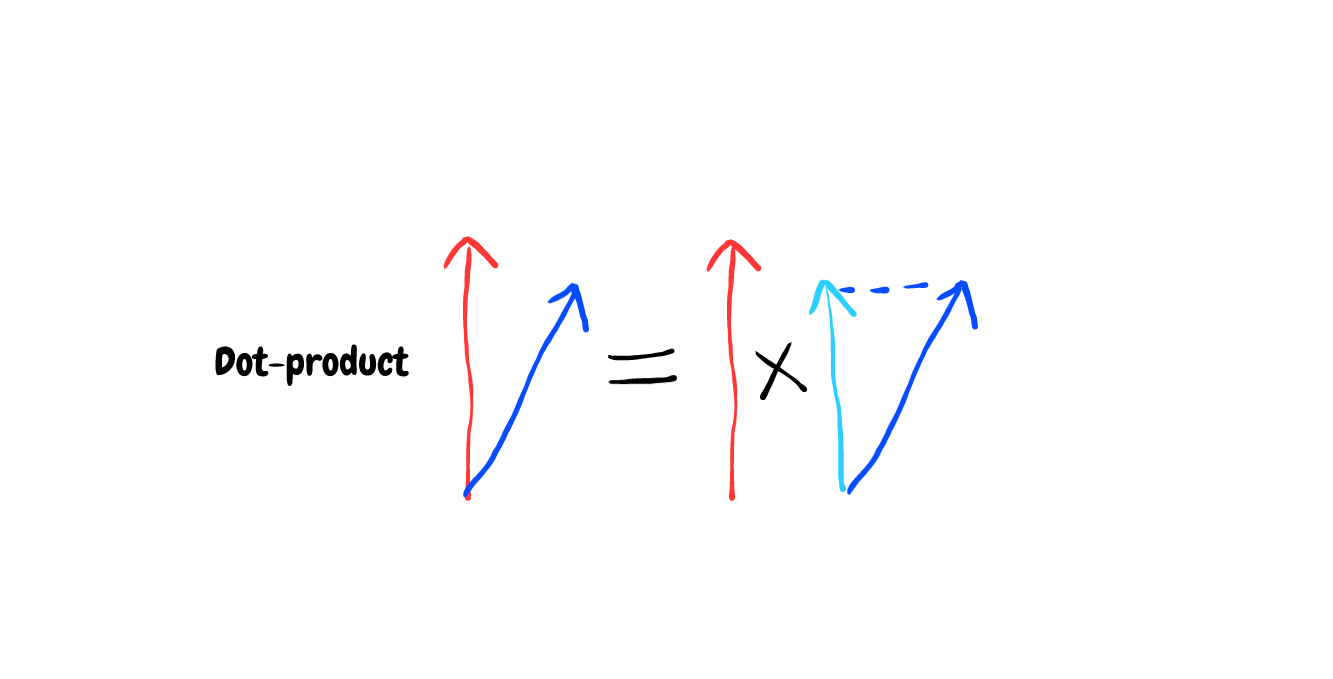
But what about the dot-product ? The dot-product has some relevances to the cosine that mentioned above. The dot-product in geometrical point of view is the projection of a vector to the direction of another vector and multiply them both. And the projection is calculated by multiplying the cosine of the angle between these 2 vectors. But in this simple case, the projection is just the y value if our predicted vector is (x,y) and the target vector is (0,1). And the y value decrease strictly from 1 to 0 from vector (1,0) to vector (0,1) . So the dot-product can also be a great candidate for our loss function too
In the multiclass classification problem with the target vector encoded by one-hot vector (Vector has just one 1 value and 0 for all others position). The dot-product calculation is very simple. Taking the value in the predicted vector that at its position in the target vector, we have 1. (Dot-product in algebra is just the sum of the element-wise multiplication)
v1 = np.array([0,1,0,0]) # target vector
v2 = np.array([0.2,0.3,0.1,0.4]) # predicted vector
print(sum(v1*v2))
For the Cross-Entropy Loss Function, instead of multiply the predicted vector, we multiply the logarithm of the predicted vector
print(sum(v1*np.log(v2)))
print(np.log(0.3))
In the next section, we will experiment the dot-product loss function, the cross-entropy loss function and try to invent of own loss function by changing the function applying the the predicted vector (like logarithm in the case of Cross-Entropy)
In this part, we will experiment our dot-product loss function, compare its performance with the famous cross-entropy loss function and finally, try to invent a new loss function that is comparable to the cross-entropy loss function.
The experiments use data from the Oxford-IIIT Pet Dataset and the resnet18 model from fastai2 library
This part is simply for data preparation. Puting all the images and their labels to the corresponding dataloader
from fastai2.vision.all import *
path = untar_data(URLs.PETS)
items = get_image_files(path/'images')
def label_func(fname):
    return "cat" if fname.name[0].isupper() else "dog"
labeller = RegexLabeller(pat=r"(.+)_\d+.jpg")
pets = DataBlock(blocks=(ImageBlock, CategoryBlock),
                    get_items=get_image_files,
                    splitter=RandomSplitter(),
                    get_y = Pipeline([lambda x: getattr(x,'name'), labeller]),
                    item_tfms=Resize(224),
                    batch_tfms=aug_transforms(),
                    )
dls = pets.dataloaders(path/'images')
dls.c # number of categories in this dataset
dls.show_batch()

All our loss functions will have two parts. The first part is the softmax function - scaling our output to [0,1] and. The second part is the how we penalize our prediction - high loss if the predicted vector is far from the target.
def softmax(x): return x.exp() / (x.exp().sum(-1)).unsqueeze(-1)
def nl(input, target): return -input[range(target.shape[0]), target].log().mean()
def our_cross_entropy(input, target):
    pred = softmax(input)
    loss = nl(pred, target)
    return loss
learn = cnn_learner(dls, resnet18, loss_func=our_cross_entropy, metrics=error_rate)
learn.fine_tune(1)
This is actually a negative dot-production loss function because we multiply the result to -1 to make it increasing from best to worst prediction
def dot_product_loss(input, target):
    pred = softmax(input)
    return -(pred[range(target.shape[0]), target]).mean()
learn = cnn_learner(dls, resnet18, loss_func=dot_product_loss, metrics=error_rate)
learn.fine_tune(1)
Wow ! despite the simplicity of the dot-product loss function, we got not so bad result (0.14) after 2 epochs. Our dataset has 37 categories of pets and a random prediction will give us the error rate (1-1/37)=0.97. However, can we do it better, somehow geting closer to the performance of the cross-entropy loss function ?
How these 2 loss functions penalize the prediction described as below. The target vector is always [0,1]
x = np.linspace(0.01,0.99,100) # the predicted vector at index 2
y_dot_product = -x
y_cross_entropy = -np.log(x)
plt.plot(x, y_dot_product, label='dot_prod')
plt.plot(x, y_cross_entropy, label='cross_entropy')
plt.legend()
plt.show()

The shape of the plot is what we interested here. Intuitively, we can see that the cross-entropy function penalize more when we have wrong prediction (kind of exponential shape), maybe it cause the better prediction
In the next section we will try other loss function but the core idea is still based on the dot-product loss function.
Instead of multiply by -1, we can inverse the predicted value to make it increasing from best to worst prediction. Let's see the plot as below:
y_inv = 1/x
plt.plot(x, y_dot_product, label='dot_prod')
plt.plot(x, y_cross_entropy, label='cross_entropy')
plt.plot(x, y_inv, label='inverse loss')

plt.legend()
plt.show()

Hmmm! The inverse loss penalize may be too much compared to the 2 previous ones, no tolerance at all might be not so good. But let's try it anyway
def inverse_loss(input, target):
    pred = softmax(input)
    return (1/((pred[range(target.shape[0]), target]))).mean()
learn = cnn_learner(dls, resnet18, loss_func=inverse_loss, metrics=error_rate)
learn.fine_tune(1)
Ok, we have worst result. But with this idea, we can easily tunning the loss function. We can power the denominator with value < 1 to decrease the penalization. For example: 0.2
y_inv_tuning = 1/(x**0.2)
plt.plot(x, y_dot_product, label='dot_prod')
plt.plot(x, y_cross_entropy, label='cross_entropy')
plt.plot(x, y_inv_tuning, label='inverse loss tuning')

plt.legend()
plt.show()

Great! Let's try this new loss function
def inverse_loss_tunning(input, target):
    pred = softmax(input)
    return (1/((pred[range(target.shape[0]), target]).pow(0.2))).mean()
learn = cnn_learner(dls, resnet18, loss_func=inverse_loss_tunning, metrics=error_rate)
learn.fine_tune(1)
We get not so different error rate: 0.091 compared to 0.092 of the cross-entropy loss function.
I hope after reading this blog, you can understand deeper the loss function of multi-classes classification problem. My purpose is not actually finding a new loss function to replace the cross-entropy, but give you an idea of how to define you own in maybe another problem. And I also want to remind (for you and even for myself) that in machine learning, your intuition, or your sense, counts. I developed all the experiments above just from my natual intuition, and the most popular approach everybody use may not be the best approach and you can not change it. While following the fastai course, I found a story about Learning Rate Finder from Leslie Smith which is developped not long ago (2015), and it doesn't use very advanced math. So be patient, be brave and be creative to follow the Deep Learning road.