dhblog - Transformer for timeseries

Developing an Intuition for Transformers and Applying Them to Time Series Classification

Struggling to learn a new deep learning architecture, such as Transformer, can be quite challenging. However, it doesn’t have to be so daunting. In this blog post, I will demonstrate a practical approach to start using a new architecture, specifically the Transformer. We will construct a basic Transformer architecture and progressively fine-tune it to achieve the performance of the TST architecture (A Transformer-based Framework for Multivariate Time Series Representation Learning).

Content:

Dataset to use: FaceDetection
Reference Model: TST Model implemented in tsai repository
Baseline Model: LSTM Model
Our Simple TST Model
Improvement

References:

You’ll need fastai and tsai to run the code in this blog-post

!pip install -Uqq tsai

import torch
from torch.utils.data import Dataset
from torch import nn
from fastai.data.core import DataLoader, DataLoaders
from fastai.learner import Learner
from fastai.losses import LabelSmoothingCrossEntropyFlat
from fastai.metrics import RocAucBinary, accuracy
from fastai.torch_core import Module
from fastai.layers import Flatten
from tsai.models.TST import TST
from tsai.models.RNN import LSTM
from tsai.data.external import get_UCR_data
from tsai.callback.core import ShowGraph as ShowGraphCallback2
from tsai.learner import plot_metrics
from tsai.imports import default_device
import numpy as np
from torch.nn.modules.transformer import TransformerEncoderLayer, TransformerEncoder

Dataset: FaceDetection

Note

Why Time Series? Although the Transformer originates from the NLP domain and outperforms all previous architectures, I believe that, for those not yet familiar with NLP, it is more advantageous to start with a domain that requires less preprocessing, such as Time Series. This way, we can focus our attention on understanding the architecture itself.

In this tutorial, we will be using a dataset from the well-known UEA & UCR Time Series repository. Although we won’t delve into the details of this dataset in this blog post, it’s worth mentioning its purpose. The objective is to classify whether a given MEG signal (Magnetoencephalography) represents a face or not. The input dimension is 144, and the sequence length is 62.

I chose this dataset because it contains a reasonable amount of data (5,890 training instances and 3,524 testing instances) and has been used in a Transformer tutorial in the tsai repository. This ensures that we have a reliable reference model to aim to outperform.

We will utilize utility functions from the tsai and fastai libraries to facilitate our work and streamline the process.

batch_size, c_in, c_out, seq_len = 64, 144, 2, 62
X, y, splits = get_UCR_data('FaceDetection', return_split=False)

X_train = X[splits[0]]
y_train = y[splits[0]]
X_valid = X[splits[1]]
y_valid = y[splits[1]]

mean_trn = np.mean(X_train, axis=(0,2), keepdims=True)
std_trn = np.std(X_train, axis=(0,2), keepdims=True)

class TSDataset(Dataset):
    """TimeSeries DataSet for FaceDetection"""
    def __init__(self, X, y):
        super(TSDataset, self).__init__()
        self.X = torch.tensor(X)
        self.Y = torch.concat([torch.tensor([_y == '0'], dtype=int) for _y in y])
    
    def __len__(self): return len(self.X)
    
    def __getitem__(self, i):
        return self.X[i], self.Y[i]

The following code demonstrates how to create data loaders for the training and validation sets:

dset_train = TSDataset(X_train, y_train)
dset_valid = TSDataset(X_valid, y_valid)

dl_train = DataLoader(dset_train, batch_size=batch_size, shuffle=True)
dl_valid = DataLoader(dset_valid, batch_size=batch_size, shuffle=False)

dls = DataLoaders(dl_train, dl_valid) 
dls = dls.cuda()

x, y = next(iter(dl_train))

x.shape, y.shape

(torch.Size([64, 144, 62]), torch.Size([64]))

Reference Model

The reference model we will be using is the TST (Transformer-based Framework for Multivariate Time Series Representation Learning) and implemented by the tsai library.

def evaluate_model(model, n_epoch=30):
    learn = Learner(dls, model, loss_func=LabelSmoothingCrossEntropyFlat(), 
                    metrics=[RocAucBinary(), accuracy],  cbs=ShowGraphCallback2())
    learn.fit_one_cycle(n_epoch, 1e-4)

model = TST(c_in, c_out, seq_len, dropout=0.3, fc_dropout=0.9, n_heads=1, n_layers=1)

evaluate_model(model)

epoch	train_loss	valid_loss	roc_auc_score	accuracy	time
0	0.943482	0.710201	0.503936	0.505675	00:02
1	0.959244	0.705551	0.515424	0.515607	00:01
2	0.940436	0.697859	0.534342	0.532350	00:01
3	0.900420	0.692391	0.563204	0.543133	00:01
4	0.872391	0.682138	0.601740	0.567537	00:01
5	0.873357	0.674679	0.632084	0.591090	00:01
6	0.827063	0.668141	0.662991	0.618331	00:01
7	0.802059	0.658147	0.682879	0.635925	00:01
8	0.753277	0.653781	0.693962	0.641884	00:01
9	0.744286	0.647927	0.698235	0.643303	00:01
10	0.727256	0.646205	0.705161	0.654370	00:01
11	0.699470	0.644024	0.707230	0.654654	00:01
12	0.707701	0.639246	0.713946	0.663167	00:01
13	0.677575	0.637510	0.716578	0.663734	00:01
14	0.690399	0.635938	0.720142	0.667991	00:01
15	0.651648	0.635806	0.720622	0.667991	00:01
16	0.639079	0.634356	0.722736	0.665153	00:01
17	0.672199	0.633124	0.724921	0.665437	00:01
18	0.639468	0.631378	0.728070	0.668558	00:01
19	0.638936	0.629368	0.728399	0.668558	00:01
20	0.625763	0.627779	0.731610	0.672247	00:01
21	0.619361	0.626804	0.732947	0.671680	00:01
22	0.633200	0.626732	0.732423	0.673666	00:01
23	0.633324	0.625232	0.735347	0.673099	00:01
24	0.639257	0.625497	0.733850	0.672531	00:01
25	0.626306	0.625547	0.733988	0.671396	00:01
26	0.616693	0.625246	0.734917	0.674234	00:01
27	0.627592	0.625567	0.733930	0.671396	00:01
28	0.616872	0.625370	0.734323	0.671680	00:01
29	0.617217	0.624772	0.734979	0.672815	00:01

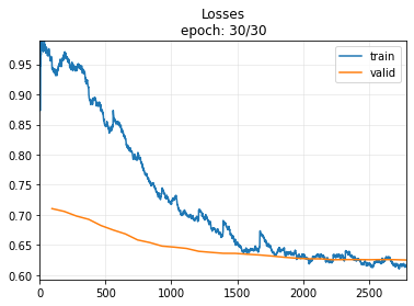
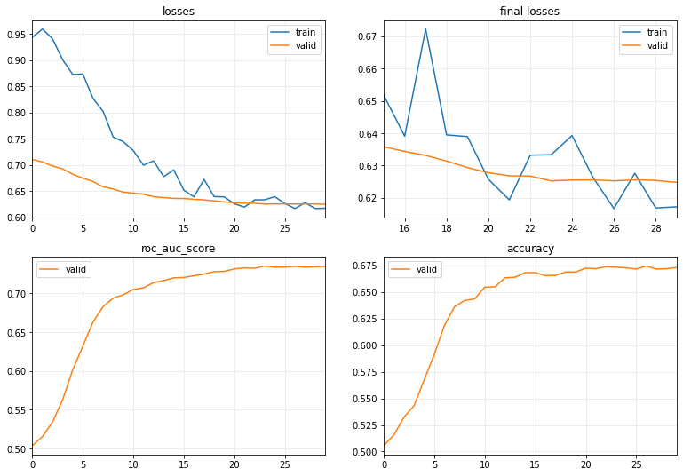
Note

For the simplicity for the reader, I do not use any normalization technique and training in lesser number of epochs than the original reference notebook. After 100 epochs, they reach an accuracy arount 0.70.1

Baseline

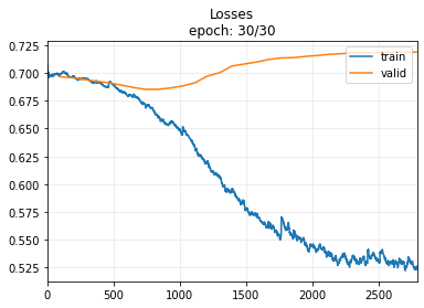
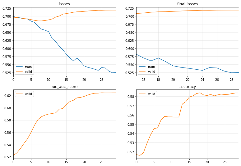
We’ll begin our journey by exploring an LSTM model, which was commonly used for sequence classification in the pre-transformer era.

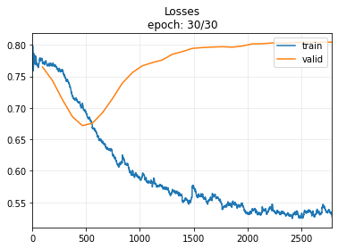
Note

Note: Observing the validation loss may lead you to believe that the model is overfitting. However, this is not the case, as the final metric (accuracy) continues to increase.

model = LSTM(144,2,rnn_dropout=0.3, fc_dropout=0.3)

evaluate_model(model)

epoch	train_loss	valid_loss	roc_auc_score	accuracy	time
0	0.698941	0.696725	0.522427	0.517026	00:02
1	0.696502	0.695753	0.526428	0.516175	00:01
2	0.694726	0.694219	0.533478	0.519013	00:01
3	0.691055	0.692617	0.541788	0.529228	00:01
4	0.691306	0.691157	0.549403	0.538309	00:01
5	0.684514	0.689195	0.559889	0.545119	00:01
6	0.680696	0.686942	0.571706	0.545970	00:01
7	0.668403	0.685266	0.581042	0.554767	00:01
8	0.659610	0.685288	0.585615	0.558456	00:01
9	0.656271	0.686517	0.588135	0.557889	00:01
10	0.651706	0.688422	0.589830	0.557889	00:01
11	0.630258	0.691245	0.590714	0.557605	00:01
12	0.620531	0.697241	0.591923	0.557605	00:01
13	0.606660	0.700341	0.597773	0.571793	00:01
14	0.595829	0.706305	0.598964	0.574347	00:01
15	0.581478	0.708097	0.604908	0.579455	00:01
16	0.570084	0.709881	0.610240	0.580590	00:01
17	0.560884	0.712225	0.612305	0.583144	00:01
18	0.570109	0.713588	0.616308	0.583995	00:01
19	0.558659	0.713829	0.616927	0.581725	00:01
20	0.545606	0.714969	0.618493	0.580874	00:01
21	0.541346	0.715872	0.620730	0.582293	00:01
22	0.538415	0.716904	0.622545	0.580590	00:01
23	0.535115	0.717429	0.623803	0.581725	00:01
24	0.531399	0.718325	0.623906	0.582577	00:01
25	0.540339	0.718253	0.624539	0.582009	00:01
26	0.539049	0.718644	0.624380	0.582293	00:01
27	0.529248	0.718712	0.624360	0.583144	00:01
28	0.524167	0.718756	0.624453	0.583712	00:01
29	0.524851	0.718751	0.624465	0.583712	00:01

Our TST

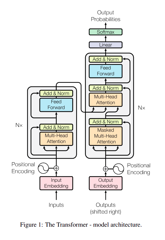
The diagram above illustrates the Transformer architecture as presented in the “Attention is All You Need” paper. The breakthrough in this architecture is the Multi-Head Attention. The idea behind Attention is that if your model can focus on the most important parts of a long sequence, it can perform better without being affected by noise.

How does it work? Well, in my experience, when we are not very familiar with a new architecture, we shouldn’t focus too much on understanding every detail of the architecture. I spent a lot of time reading various tutorials, trying to grasp the clever idea behind this, only to realize that I still didn’t know how to apply it to a real case. I will attempt to cover building Self-Attention from scratch in a future blog post. However, in this one, we will start by learning how to use the Transformer module from PyTorch.

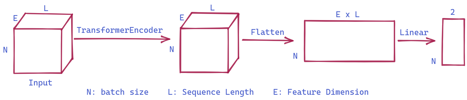
What do we need to pay attention to here? We will mainly focus on the shapes of the input and output. The input maintains its shape after passing through the Transformer Encoder. Subsequently, the output is flattened and passed through a linear layer, which generates the appropriate number of classes for the given classification task

Our first model as below is a very simple architecture with just one TransformerEncoder Layer and one Linear Layer

batch_size, c_in, d_model, c_out, seq_len, dropout, fc_dropout  = 64, 144, 128, 2, 62, 0.7, 0.9

class OurTST(Module):
    def __init__(self, c_in, c_out, seq_len, dropout):
        self.c_in, self.c_out, self.seq_len = c_in, c_out, seq_len
        encoder_layer = TransformerEncoderLayer(d_model=c_in, nhead=1, dropout=dropout)
        self.transformer_encoder = TransformerEncoder(encoder_layer, num_layers=1)
        self.head = nn.Linear(seq_len*c_in, c_out)
    def forward(self, x):
        o = x.swapaxes(1,2) # [bs,c_in,seq_len] -> [bs,seq_len,c_in]
        o = self.transformer_encoder(o) # [bs,c_in,seq_len] -> [bs,c_in,seq_len]
        o = o.reshape(o.shape[0], -1) # [bs,c_in,seq_len] -> [bs,c_in x seq_len]
        o = self.head(o) # [bs,c_in x seq_len] -> [bs,]
        return o

model = OurTST(c_in, c_out, seq_len, 0.9)

model

OurTST(
  (transformer_encoder): TransformerEncoder(
    (layers): ModuleList(
      (0): TransformerEncoderLayer(
        (self_attn): MultiheadAttention(
          (out_proj): NonDynamicallyQuantizableLinear(in_features=144, out_features=144, bias=True)
        )
        (linear1): Linear(in_features=144, out_features=2048, bias=True)
        (dropout): Dropout(p=0.9, inplace=False)
        (linear2): Linear(in_features=2048, out_features=144, bias=True)
        (norm1): LayerNorm((144,), eps=1e-05, elementwise_affine=True)
        (norm2): LayerNorm((144,), eps=1e-05, elementwise_affine=True)
        (dropout1): Dropout(p=0.9, inplace=False)
        (dropout2): Dropout(p=0.9, inplace=False)
      )
    )
  )
  (head): Linear(in_features=8928, out_features=2, bias=True)
)

evaluate_model(model, 30)

epoch	train_loss	valid_loss	roc_auc_score	accuracy	time
0	0.771023	0.765103	0.501380	0.503405	00:01
1	0.767232	0.743445	0.526820	0.517877	00:01
2	0.760522	0.713145	0.577938	0.552781	00:01
3	0.718567	0.686044	0.636998	0.599603	00:01
4	0.707388	0.671847	0.679890	0.627128	00:01
5	0.667916	0.675715	0.702388	0.650114	00:01
6	0.646124	0.692107	0.713854	0.657492	00:01
7	0.626370	0.714405	0.720573	0.665153	00:01
8	0.623622	0.739222	0.721124	0.671396	00:01
9	0.597921	0.755921	0.722508	0.669410	00:01
10	0.595011	0.766809	0.725383	0.672815	00:01
11	0.574535	0.771822	0.729465	0.675936	00:01
12	0.573907	0.776058	0.732046	0.671112	00:01
13	0.570190	0.785060	0.733693	0.673950	00:01
14	0.552551	0.789218	0.734351	0.674234	00:01
15	0.575410	0.794398	0.736869	0.678774	00:01
16	0.563437	0.795728	0.738365	0.676788	00:01
17	0.563861	0.796549	0.739659	0.680193	00:01
18	0.538637	0.797076	0.740454	0.679909	00:01
19	0.548644	0.796367	0.741566	0.681896	00:01
20	0.549104	0.798111	0.741827	0.685017	00:01
21	0.539753	0.801571	0.741463	0.683598	00:01
22	0.542557	0.801905	0.742229	0.683031	00:01
23	0.547139	0.803032	0.742469	0.682463	00:01
24	0.532426	0.802947	0.743231	0.683598	00:01
25	0.524330	0.803357	0.743226	0.683314	00:01
26	0.525560	0.803959	0.743130	0.683598	00:01
27	0.534251	0.804135	0.743205	0.682747	00:01
28	0.541934	0.804315	0.743135	0.682747	00:01
29	0.527424	0.804290	0.743156	0.682747	00:01

Well, our model outperforms the LSTM model and even better than the TST model after 30 epochs

Upgrades

In this section, I will discuss how we can build upon our basic Transformer architecture to achieve even greater results. We will explore several ideas inspired by the original paper and general deep learning concepts.

1- Feature Standardizing:

To enhance neural network training, it is recommended that input data have a zero mean and unit standard deviation ( for more details, refer to this lesson from fast.ai). In line with the original paper, we employ feature standardization, which standardizes each feature separately.

mean_trn = np.mean(X_train, axis=(0,2), keepdims=True)
std_trn = np.std(X_train, axis=(0,2), keepdims=True)
... # In the Dataset
self.X = (self.X - mean_trn)/std_trn

2- Input Projection

Before feeding the input into the TransformerEncoder layer, it can be projected into another dimension, allowing us to control the input received by the TransformerEncoder. In general, using suitable techniques, a deeper network can potentially outperform a shallow one.

    def __init__( ... )
        self.W_P = nn.Linear(c_in, d_model)
    def forward(self, x):
        o = x.swapaxes(1, 2)  
        o = self.W_P(o)  # Input Projection

3- Positional Encoding

Transformers do not inherently capture the positional order of input data, which can be crucial for certain tasks. To embed this information, we can employ techniques such as passing the input through a specific function (e.g., a sinusoidal function) or creating learnable parameters for position (as implemented in our code).

    def __init__( ... )
        # Positional encoding
        W_pos = torch.empty((seq_len, d_model), device=default_device())
        nn.init.uniform_(W_pos, -0.02, 0.02)
        self.W_pos = nn.Parameter(W_pos, requires_grad=True)
    def forward(self, x):
        o = x.swapaxes(1, 2)  
        o = self.W_P(o)  
        o = o + self.W_pos # Positional Encoding

4- DropOut

Deep neural networks can be prone to overfitting. To mitigate this issue, we can introduce dropout layers in our model, making it more resistant to overfitting. In our architecture, there are two types of dropout: one within the TransformerEncoder layer and another just before the final Linear layer.

    def __init__( ... )
        # Transformer encoder layers
        encoder_layer = TransformerEncoderLayer(d_model=d_model, nhead=1, dropout=drop_out) # dropout inside Transformer Layer
        self.transformer_encoder = TransformerEncoder(encoder_layer, num_layers=n_layers)

        self.head = nn.Sequential(
            nn.GELU(),
            Flatten(),
            nn.Dropout(fc_dropout), # fully connected dropout
            nn.Linear(seq_len * d_model, c_out)
        )

batch_size, c_in, d_model, c_out, seq_len,fc_dropout = 64, 144, 128, 2, 62, 0.9
X, y, splits = get_UCR_data('FaceDetection', return_split=False)

X_train = X[splits[0]]
y_train = y[splits[0]]
X_valid = X[splits[1]]
y_valid = y[splits[1]]

mean_trn = np.mean(X_train, axis=(0,2), keepdims=True)
std_trn = np.std(X_train, axis=(0,2), keepdims=True)

class TSDataset(Dataset):
    """TimeSeries DataSet for FaceDetection"""
    def __init__(self, X, y):
        super(TSDataset, self).__init__()
        self.X = torch.tensor(X)
        self.X = (self.X - mean_trn)/std_trn
        self.Y = torch.concat([torch.tensor([_y == '0'], dtype=int) for _y in y])
    
    def __len__(self): return len(self.X)
    
    def __getitem__(self, i):
        return self.X[i], self.Y[i]

class OurTST(Module):
    def __init__(self, c_in, c_out, d_model, seq_len, n_layers, drop_out, fc_dropout):
        self.c_in, self.c_out, self.seq_len = c_in, c_out, seq_len
        self.W_P = nn.Linear(c_in, d_model)

        # Positional encoding
        W_pos = torch.empty((seq_len, d_model), device=default_device())
        nn.init.uniform_(W_pos, -0.02, 0.02)
        self.W_pos = nn.Parameter(W_pos, requires_grad=True)

        # Transformer encoder layers
        encoder_layer = TransformerEncoderLayer(d_model=d_model, nhead=1, dropout=drop_out)
        self.transformer_encoder = TransformerEncoder(encoder_layer, num_layers=n_layers)

        self.head = nn.Sequential(
            nn.GELU(),
            Flatten(),
            nn.Dropout(fc_dropout),
            nn.Linear(seq_len * d_model, c_out)
        )

    def forward(self, x):
        o = x.swapaxes(1, 2)  # [bs,c_in,seq_len] -> [bs,seq_len,c_in]
        o = self.W_P(o)  # [bs,seq_len,c_in] -> [bs,seq_len,d_model]
        o = o + self.W_pos
        o = self.transformer_encoder(o)  # [bs, seq_len, d_model] -> [bs, seq_len, d_model]
        o = o.contiguous()
        o = self.head(o)  # [bs,seq_len x d_model] -> [bs,c_out]
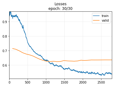
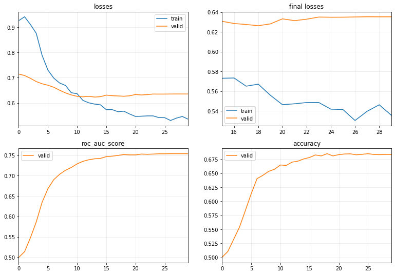
        return o

model = OurTST(c_in, c_out, d_model, seq_len, 3, 0.4 ,0.9)

evaluate_model(model, n_epoch=30)

epoch	train_loss	valid_loss	roc_auc_score	accuracy	time
0	0.925684	0.714104	0.499395	0.500000	00:02
1	0.941063	0.708397	0.513332	0.510499	00:02
2	0.910563	0.697380	0.547459	0.532066	00:02
3	0.875563	0.684338	0.586375	0.553916	00:02
4	0.788294	0.675705	0.634576	0.583144	00:02
5	0.729792	0.669882	0.668022	0.613224	00:02
6	0.698079	0.661823	0.690192	0.640182	00:02
7	0.678686	0.650137	0.703406	0.646141	00:02
8	0.669151	0.639466	0.713121	0.653235	00:02
9	0.640111	0.631399	0.720097	0.656924	00:02
10	0.636223	0.625919	0.728919	0.664586	00:02
11	0.609655	0.623980	0.735162	0.663734	00:02
12	0.600260	0.626050	0.739055	0.669694	00:02
13	0.595127	0.623003	0.741405	0.671396	00:02
14	0.592127	0.624625	0.742487	0.675369	00:02
15	0.572983	0.630688	0.746745	0.677923	00:02
16	0.573267	0.628453	0.747862	0.682463	00:02
17	0.564986	0.627425	0.749735	0.680761	00:02
18	0.567010	0.626230	0.751817	0.684733	00:02
19	0.555792	0.628040	0.751030	0.680761	00:02
20	0.546230	0.633149	0.751046	0.683031	00:02
21	0.547146	0.631326	0.752979	0.684166	00:02
22	0.548416	0.632791	0.752416	0.684449	00:02
23	0.548463	0.634959	0.752966	0.682747	00:02
24	0.541696	0.634788	0.753698	0.683598	00:02
25	0.541297	0.634837	0.753692	0.684733	00:02
26	0.530234	0.635058	0.753956	0.683314	00:02
27	0.539544	0.635267	0.753939	0.683031	00:02
28	0.546123	0.635198	0.753946	0.683314	00:02
29	0.535531	0.635230	0.753916	0.683314	00:02

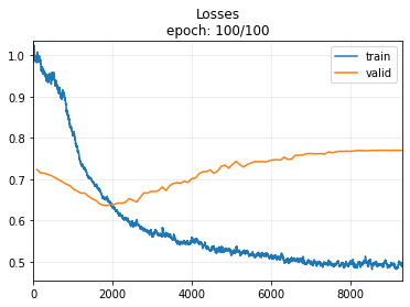
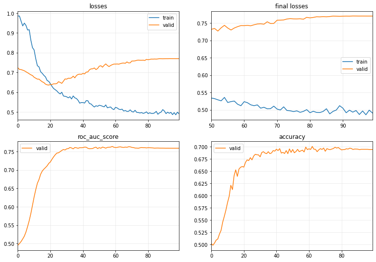
Let’s try training with more epochs. In the following example, we will train for 100 epochs, which is the same as in this tutorial from tsai

model = OurTST(c_in, c_out, d_model, seq_len, 3, 0.6 ,0.9)
evaluate_model(model, n_epoch=100)

epoch	train_loss	valid_loss	roc_auc_score	accuracy	time
0	0.986113	0.723611	0.495537	0.501986	00:02
1	0.985938	0.715433	0.500191	0.498581	00:02
2	0.959804	0.714567	0.505571	0.503121	00:02
3	0.935837	0.711624	0.512527	0.509081	00:02
4	0.949967	0.708520	0.520180	0.511351	00:02
5	0.938500	0.703618	0.531381	0.521283	00:02
6	0.914983	0.698704	0.546194	0.528944	00:02
7	0.916452	0.693311	0.562272	0.545687	00:02
8	0.863562	0.688229	0.581601	0.557605	00:02
9	0.825720	0.684290	0.603750	0.570658	00:02
10	0.814094	0.675768	0.626344	0.585982	00:02
11	0.770269	0.671013	0.646063	0.598751	00:02
12	0.734332	0.666361	0.663611	0.621169	00:02
13	0.728247	0.666351	0.673837	0.612372	00:02
14	0.703636	0.659145	0.688090	0.640749	00:02
15	0.695590	0.652872	0.696829	0.652667	00:02
16	0.685371	0.648839	0.701994	0.639330	00:02
17	0.677378	0.640827	0.706331	0.654370	00:02
18	0.659291	0.637410	0.711023	0.658059	00:02
19	0.654945	0.636273	0.717630	0.659478	00:02
20	0.642616	0.639057	0.721688	0.658343	00:02
21	0.629476	0.639091	0.728980	0.667991	00:02
22	0.618588	0.642530	0.735525	0.673099	00:02
23	0.612620	0.642298	0.741208	0.671680	00:02
24	0.606063	0.644125	0.745705	0.677639	00:02
25	0.597042	0.653301	0.746442	0.673099	00:02
26	0.591410	0.649610	0.749507	0.680761	00:02
27	0.599989	0.644790	0.752807	0.684449	00:02
28	0.580830	0.655860	0.755328	0.683598	00:02
29	0.579203	0.667195	0.754020	0.683314	00:02
30	0.576821	0.666351	0.757188	0.679342	00:02
31	0.571501	0.670810	0.757713	0.688138	00:02
32	0.577291	0.670262	0.760897	0.689841	00:02
33	0.565669	0.672775	0.759541	0.687003	00:02
34	0.581174	0.681387	0.757111	0.685868	00:02
35	0.571533	0.672656	0.760768	0.689841	00:02
36	0.568005	0.684501	0.759986	0.685868	00:02
37	0.558923	0.689911	0.758634	0.687287	00:02
38	0.544595	0.691652	0.760238	0.692111	00:02
39	0.547767	0.690527	0.760010	0.690976	00:02
40	0.547662	0.695285	0.760551	0.694949	00:02
41	0.545006	0.692685	0.761823	0.692111	00:02
42	0.557433	0.701815	0.761501	0.696084	00:02
43	0.556936	0.702578	0.758627	0.687003	00:02
44	0.542515	0.713648	0.757356	0.688422	00:02
45	0.540261	0.718203	0.757706	0.686152	00:02
46	0.531610	0.718681	0.758163	0.692111	00:02
47	0.525029	0.722788	0.760487	0.685868	00:02
48	0.531557	0.714598	0.761604	0.695516	00:02
49	0.528427	0.720070	0.757874	0.688422	00:02
50	0.533936	0.731660	0.760347	0.694381	00:02
51	0.532107	0.734147	0.758814	0.687571	00:02
52	0.528784	0.726680	0.761935	0.690125	00:02
53	0.525845	0.736096	0.760733	0.694665	00:02
54	0.535664	0.743276	0.758939	0.689841	00:02
55	0.521018	0.735471	0.761122	0.691544	00:02
56	0.523641	0.729754	0.761421	0.692963	00:02
57	0.525150	0.735508	0.761838	0.689274	00:02
58	0.516105	0.739418	0.763721	0.699205	00:02
59	0.511782	0.742465	0.761415	0.694098	00:02
60	0.523468	0.742341	0.760741	0.695800	00:02
61	0.520403	0.743021	0.761011	0.694381	00:02
62	0.514355	0.741946	0.762210	0.700624	00:02
63	0.511770	0.744806	0.762579	0.694949	00:02
64	0.514207	0.747035	0.761403	0.694665	00:02
65	0.504732	0.747706	0.760959	0.689841	00:02
66	0.507337	0.746426	0.761844	0.693530	00:02
67	0.502984	0.753452	0.761258	0.696084	00:02
68	0.503284	0.748423	0.762783	0.694381	00:02
69	0.510511	0.748741	0.762635	0.697219	00:02
70	0.502065	0.757950	0.761098	0.690692	00:02
71	0.499528	0.758117	0.760646	0.696084	00:02
72	0.508516	0.758758	0.759330	0.694665	00:02
73	0.497975	0.761433	0.759172	0.694098	00:02
74	0.497121	0.762476	0.758746	0.695233	00:02
75	0.494813	0.761791	0.759932	0.696368	00:02
76	0.496914	0.761701	0.760781	0.698922	00:02
77	0.492758	0.762113	0.760283	0.697219	00:02
78	0.495429	0.760835	0.760252	0.698354	00:02
79	0.500510	0.766248	0.759687	0.695800	00:02
80	0.491652	0.764638	0.760198	0.693530	00:02
81	0.495746	0.766025	0.760069	0.694098	00:02
82	0.492518	0.767861	0.759896	0.694381	00:02
83	0.492122	0.767575	0.759625	0.695800	00:02
84	0.495317	0.768247	0.758977	0.695233	00:02
85	0.503044	0.767743	0.759250	0.696935	00:02
86	0.488295	0.768618	0.759364	0.696368	00:02
87	0.495461	0.769804	0.759051	0.694381	00:02
88	0.499347	0.769520	0.758997	0.695233	00:02
89	0.511932	0.769175	0.758995	0.695233	00:02
90	0.504696	0.769521	0.758882	0.694949	00:02
91	0.491524	0.769784	0.758762	0.694098	00:02
92	0.498932	0.769638	0.758810	0.694665	00:02
93	0.493265	0.770175	0.758754	0.694665	00:02
94	0.497908	0.770099	0.758764	0.694665	00:02
95	0.486489	0.769981	0.758742	0.694665	00:02
96	0.496604	0.770035	0.758724	0.694665	00:02
97	0.485646	0.769963	0.758733	0.694381	00:02
98	0.499033	0.769941	0.758741	0.694381	00:02
99	0.490694	0.769939	0.758742	0.694381	00:02

Note

There may be differences between the implementation of the Transformer in pytorch and tsai (for example, pytorch uses LayerNorm in the TransformerEncoder layer, which is popular in NLP, while tsai employs BatchNorm)