dhblog - Object Detection from scratch

Building an Object Detection from scratch with fastai v2

Recently, I had a project that needs to modify an Object Detection Architecture. However, when I searched for related repositories, I found it quite difficult to understand. We have a lot of libraries for use out of the box but hard to make changes to the source code.

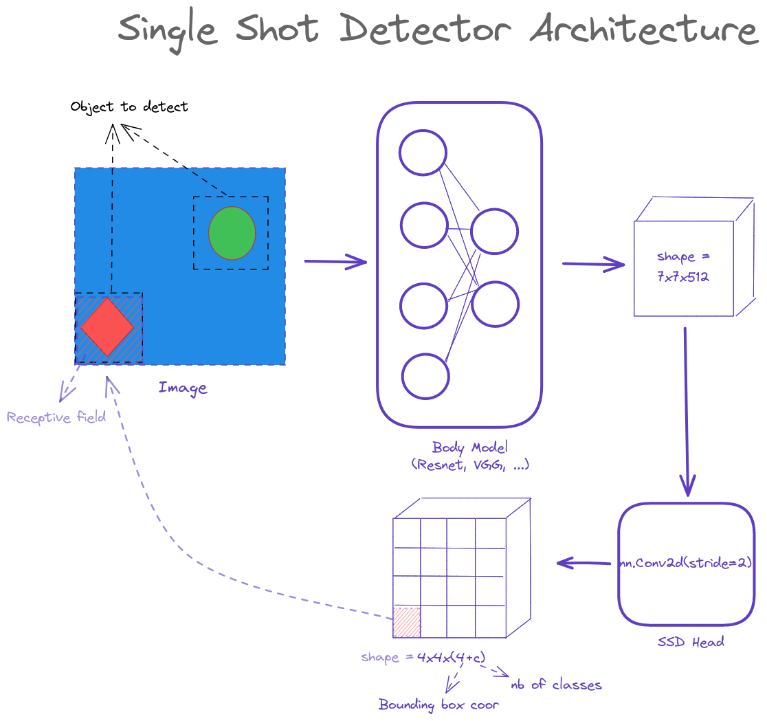
This blog is the implementation of Single Shot Detector Architecture using fast.ai in literate programming style so the readers can follow and run each line of code themselves in case needed to deepen their knowledge.

The original idea was taken from the fastai 2018 course. Readers are recommended to watch this lecture. 2018 Lecture

Some useful notes taken by students: - Cedrick Note - Francesco Note

Dataset used: Pascal 2017

What we can learn from this notebook:

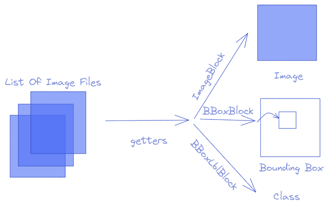
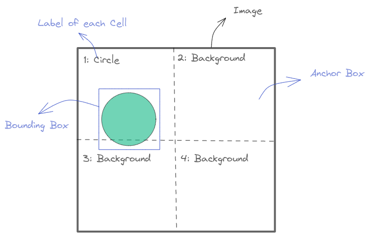
Object Detection DataLoaders from fastai DataBlock which contains Image, Bounding Box and Label. Understanding how the data resemble
Building Single Shot Detector (SSD) - Object Detection Model
Simple 4x4 Anchor Boxes. Relation between Receptive field and Anchor Boxes.
Loss function, Visualize Match to Ground-Truth
Classification Loss Discussion: Binary Cross Entropy and why Focal Loss is better
More Anchor Boxes: 3 layers of grids ( 4x4, 2x2, 1x1 ) with 9 variations (Zoom,Scale) / cell
Training and Results
Cleaning predictions with Non Maximum Supression (NMS)

%load_ext autoreload
%autoreload 2

from fastai.vision.all import *

/home/ubuntu/miniconda3/envs/blog/lib/python3.10/site-packages/tqdm/auto.py:22: TqdmWarning: IProgress not found. Please update jupyter and ipywidgets. See https://ipywidgets.readthedocs.io/en/stable/user_install.html
  from .autonotebook import tqdm as notebook_tqdm

Object Detection Dataloaders

For objection detection, you have:

1 independent variable (X): Image
2 dependents variables (Ys): Bounding box and Class

In this part, we will use fastai DataBlock to build Object Detection Dataloaders. The idea is from each image file name, we will have:

An Image
Bounding Boxes getting from the annotations file
Labels correspond to each bounding box

Note

Zero padding: Each image have a different number of objects. Then, to make it possible to gather multiple images to one batch, the number of bounding boxes per image is the maximum in that batch (the padding value by default is 0) bb_pad
Background class: In Object Detection, we need to have a class that represents the background. fastai do it automatically for you by adding #na# at index 0
The coordinates of bounding box is rescaled to ~ -1 -> 1 in fastai/vision/core.py _scale_pnts

( Check out some outputs below for details )

path = untar_data(URLs.PASCAL_2007)

path.ls()

(#8) [Path('/home/ubuntu/.fastai/data/pascal_2007/train.json'),Path('/home/ubuntu/.fastai/data/pascal_2007/test.json'),Path('/home/ubuntu/.fastai/data/pascal_2007/test'),Path('/home/ubuntu/.fastai/data/pascal_2007/train.csv'),Path('/home/ubuntu/.fastai/data/pascal_2007/segmentation'),Path('/home/ubuntu/.fastai/data/pascal_2007/valid.json'),Path('/home/ubuntu/.fastai/data/pascal_2007/train'),Path('/home/ubuntu/.fastai/data/pascal_2007/test.csv')]

imgs, lbl_bbox = get_annotations(path/'train.json')

imgs[0], lbl_bbox[0]

('000012.jpg', ([[155, 96, 351, 270]], ['car']))

img2bbox = dict(zip(imgs, lbl_bbox))

first = {k: img2bbox[k] for k in list(img2bbox)[:1]}; first

{'000012.jpg': ([[155, 96, 351, 270]], ['car'])}

getters = [lambda o: path/'train'/o, lambda o: img2bbox[o][0], lambda o: img2bbox[o][1]]

item_tfms = [Resize(224, method='squish'),]
batch_tfms = [Rotate(), Flip(), Dihedral()]

pascal = DataBlock(blocks=(ImageBlock, BBoxBlock, BBoxLblBlock),
                 splitter=RandomSplitter(),
                 getters=getters,
                 item_tfms=item_tfms,
                 batch_tfms=batch_tfms,
                 n_inp=1)

dls = pascal.dataloaders(imgs, bs = 128)

Note

#na# is the background class as defined in BBoxLblBlock

dls.vocab

['#na#', 'aeroplane', 'bicycle', 'bird', 'boat', 'bottle', 'bus', 'car', 'cat', 'chair', 'cow', 'diningtable', 'dog', 'horse', 'motorbike', 'person', 'pottedplant', 'sheep', 'sofa', 'train', 'tvmonitor']

len(dls.vocab)

dls.show_batch()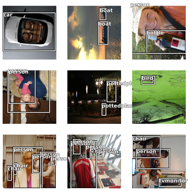

one_batch = dls.one_batch()

Note

The coordinates of boudning box is rescaled to ~ -1 -> 1 in fastai/vision/core.py

one_batch[1][0][0]

TensorBBox([-0.0440, -0.2171,  0.2200,  0.5046], device='cuda:0')

# Zero Padding
one_batch[2]

TensorMultiCategory([[13, 15,  0,  ...,  0,  0,  0],
                     [12, 15, 15,  ...,  0,  0,  0],
                     [18,  5,  5,  ...,  0,  0,  0],
                     ...,
                     [15,  8,  8,  ...,  0,  0,  0],
                     [ 7,  0,  0,  ...,  0,  0,  0],
                     [ 8,  0,  0,  ...,  0,  0,  0]], device='cuda:0')

Model Architecture

In a nutshell, Object Detection Model is a model that does 2 jobs at the same time:

a regressor with 4 outputs for bounding box
a classifier with c classes.

To handle multiple objects, here comes the grid cell. For each cell, you will have an atomic prediction for the object that dominates a part of the image ( This is the idea of the receptive field that you will see in the next part )

My Intuition

In Machine Learning, it is better to improve from something rather than start from scratch. You can see this in: Image Classification Architecture - Resnet with the Skip Connections, or Gradient Boosting in Tree-based Model. There is a common point in the grid-cell SSD architecture, the model will try to improve from an anchor box rather than searching through the whole image.

We should better leverage a well-known pretrained classification model to be used as a backbone / or body ( resnet in this tutorial ) if the object is similar to the Imagenet dataset. The head part will follow to adapt to the necessary dimension

To easily develop the idea - visualize and debug, we will start with a simple 4x4 grid

def flatten_conv(x,k):
    # Flatten the 4x4 grid to dim16 vectors
    bs,nf,gx,gy = x.size()
    x = x.permute(0,2,3,1).contiguous()
    return x.view(bs,-1,nf//k)

class OutConv(nn.Module):
    # Output Layers for SSD-Head. Contains oconv1 for Classification and oconv2 for Detection
    def __init__(self, k, nin, bias):
        super().__init__()
        self.k = k
        self.oconv1 = nn.Conv2d(nin, (len(dls.vocab))*k, 3, padding=1)
        self.oconv2 = nn.Conv2d(nin, 4*k, 3, padding=1)
        self.oconv1.bias.data.zero_().add_(bias)
        
    def forward(self, x):
        return [flatten_conv(self.oconv1(x), self.k),
                flatten_conv(self.oconv2(x), self.k)]

class StdConv(nn.Module):
    # Standard Convolutional layers 
    def __init__(self, nin, nout, stride=2, drop=0.1):
        super().__init__()
        self.conv = nn.Conv2d(nin, nout, 3, stride=stride, padding=1)
        self.bn = nn.BatchNorm2d(nout)
        self.drop = nn.Dropout(drop)
        
    def forward(self, x): return self.drop(self.bn(F.relu(self.conv(x))))

class SSD_Head(nn.Module):
    def __init__(self, k, bias):
        super().__init__()
        self.drop = nn.Dropout(0.25)
        self.sconv0 = StdConv(512,256, stride=1)
        self.sconv2 = StdConv(256,256)
        self.out = OutConv(k, 256, bias)
        
    def forward(self, x):
        x = self.drop(F.relu(x))
        x = self.sconv0(x)
        x = self.sconv2(x)
        return self.out(x)

We start with k = 1 which is the number of alterations for each anchor box ( we have a lot of anchor boxes later )

k=1

head_reg4 = SSD_Head(k, -3.)

body = create_body(resnet34(True))
model = nn.Sequential(body, head_reg4)

/home/ubuntu/miniconda3/envs/blog/lib/python3.10/site-packages/torchvision/models/_utils.py:135: UserWarning: Using 'weights' as positional parameter(s) is deprecated since 0.13 and will be removed in 0.15. Please use keyword parameter(s) instead.
  warnings.warn(
/home/ubuntu/miniconda3/envs/blog/lib/python3.10/site-packages/torchvision/models/_utils.py:223: UserWarning: Arguments other than a weight enum or `None` for 'weights' are deprecated since 0.13 and will be removed in 0.15. The current behavior is equivalent to passing `weights=ResNet34_Weights.IMAGENET1K_V1`. You can also use `weights=ResNet34_Weights.DEFAULT` to get the most up-to-date weights.
  warnings.warn(msg)

To understand and verify that everything works ok, you can take out a batch and run the model on it

out0 = body(one_batch[0].cpu())

out1 = head_reg4(out0)

out1[0].shape, out1[1].shape

(torch.Size([128, 16, 21]), torch.Size([128, 16, 4]))

Shape explanation:

128: batch size
16: number of anchor boxes
21: number of classes
4: number of bounding box coordinates

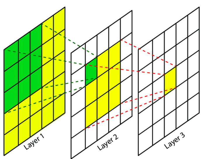
4x4 Anchor boxes and Receptive Field

As mentioned before, we will start with a 4x4 grid to better visualize the idea. The size will be normalized to [0,1]

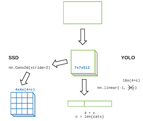
The idea of why, after the Body, we use Conv2d and not Linear Layer to make a 4x4x(4+c) output dimension instead of 16x(4+c) shape is - Receptive Field. This way, each cell will have information that comes directly from the location corresponding to the anchor box. The illustration is below.

Warning

Be very careful about the bounding box format when working with Object Detection. There are many different formats out there. For example:

pascal_voc: [x_min, y_min, x_max, y_max]
coco: [x_min, y_min, width, height]
YOLO: [x_center, y_center, width, height]

The bounding box format in this tutorial is [x_min, y_min, x_max, y_max]

Check out Bounding Boxes Augmentation for more details:

We define the anchors coordinates as below

anc_grid = 4 # Start with only 4x4 grid and no variation for each cell
k = 1 # Variation of each anchor box
anc_offset = 1/(anc_grid*2)
anc_x = np.repeat(np.linspace(anc_offset, 1-anc_offset, anc_grid), anc_grid) # Center of anc in x
anc_y = np.tile(np.linspace(anc_offset, 1-anc_offset, anc_grid), anc_grid) # Center f anc in y

anc_x

array([0.125, 0.125, 0.125, 0.125, 0.375, 0.375, 0.375, 0.375, 0.625,
       0.625, 0.625, 0.625, 0.875, 0.875, 0.875, 0.875])

anc_y

array([0.125, 0.375, 0.625, 0.875, 0.125, 0.375, 0.625, 0.875, 0.125,
       0.375, 0.625, 0.875, 0.125, 0.375, 0.625, 0.875])

anc_ctrs = np.tile(np.stack([anc_x,anc_y], axis=1), (k,1)) # Anchor centers
anc_sizes = np.array([[1/anc_grid,1/anc_grid] for i in range(anc_grid*anc_grid)])

anc_ctrs

array([[0.125, 0.125],
       [0.125, 0.375],
       [0.125, 0.625],
       [0.125, 0.875],
       [0.375, 0.125],
       [0.375, 0.375],
       [0.375, 0.625],
       [0.375, 0.875],
       [0.625, 0.125],
       [0.625, 0.375],
       [0.625, 0.625],
       [0.625, 0.875],
       [0.875, 0.125],
       [0.875, 0.375],
       [0.875, 0.625],
       [0.875, 0.875]])

anc_sizes

array([[0.25, 0.25],
       [0.25, 0.25],
       [0.25, 0.25],
       [0.25, 0.25],
       [0.25, 0.25],
       [0.25, 0.25],
       [0.25, 0.25],
       [0.25, 0.25],
       [0.25, 0.25],
       [0.25, 0.25],
       [0.25, 0.25],
       [0.25, 0.25],
       [0.25, 0.25],
       [0.25, 0.25],
       [0.25, 0.25],
       [0.25, 0.25]])

anchors = torch.tensor(np.concatenate([anc_ctrs, anc_sizes], axis=1), requires_grad=False).cuda()
# Coordinates with format: center_x, center_y, W, H

anchors

tensor([[0.1250, 0.1250, 0.2500, 0.2500],
        [0.1250, 0.3750, 0.2500, 0.2500],
        [0.1250, 0.6250, 0.2500, 0.2500],
        [0.1250, 0.8750, 0.2500, 0.2500],
        [0.3750, 0.1250, 0.2500, 0.2500],
        [0.3750, 0.3750, 0.2500, 0.2500],
        [0.3750, 0.6250, 0.2500, 0.2500],
        [0.3750, 0.8750, 0.2500, 0.2500],
        [0.6250, 0.1250, 0.2500, 0.2500],
        [0.6250, 0.3750, 0.2500, 0.2500],
        [0.6250, 0.6250, 0.2500, 0.2500],
        [0.6250, 0.8750, 0.2500, 0.2500],
        [0.8750, 0.1250, 0.2500, 0.2500],
        [0.8750, 0.3750, 0.2500, 0.2500],
        [0.8750, 0.6250, 0.2500, 0.2500],
        [0.8750, 0.8750, 0.2500, 0.2500]], device='cuda:0',
       dtype=torch.float64)

grid_sizes = torch.tensor(np.array([1/anc_grid]), requires_grad=False).unsqueeze(1).cuda()

grid_sizes

tensor([[0.2500]], device='cuda:0', dtype=torch.float64)

Visualization Utils

It is very helpful (to understand/ debug) when you can visualize data of every step. Many subtle tiny details happen in this Object Detection Problem. One careless implementation can lead to hours (or even days) to debug. Sometimes, you just wish that the code throws you some bugs that you can trackback.

Warning

There are some details that you need to double check

Are your ground truth bounding boxes, anchor boxes, bounding box activations are in the same scale ( -1 -> 1 or 0 -> 1 ) ?
Do the background class is handled correctly? ( This is a bug when I develop this notebook that the old version of the fastai course set the index of background as number_of_classes but in the latest version, it is 0 )
Do you map correctly each Anchor Box to the ground-true object? (This will be shown in the next session)

Note

Don’t hesitate to take out one batch from your dataloader and verify every single detail. When I start to use fast.ai, I made a big mistake that thinking these data are already processed and we can not show things directly from there. This data is very important, it is the input of your model. It must be carefully double-checked.

Below we will try to plot some images from a batch with their bounding boxes and classes, to see that we did not missing anything

import matplotlib.colors as mcolors
import matplotlib.cm as cmx
from matplotlib import patches, patheffects

def show_img(im, figsize=None, ax=None):
    if not ax: fig,ax = plt.subplots(figsize=figsize)
    ax.imshow(im)
    ax.set_xticks(np.linspace(0, 224, 8))
    ax.set_yticks(np.linspace(0, 224, 8))
    ax.grid()
    ax.set_yticklabels([])
    ax.set_xticklabels([])
    return ax

def draw_outline(o, lw):
    o.set_path_effects([patheffects.Stroke(
        linewidth=lw, foreground='black'), patheffects.Normal()])

def draw_text(ax, xy, txt, sz=14, color='white'):
    text = ax.text(*xy, txt,
        verticalalignment='top', color=color, fontsize=sz, weight='bold')
    draw_outline(text, 1)

def draw_rect(ax, b, color='white'):
    patch = ax.add_patch(patches.Rectangle(b[:2], *b[-2:], fill=False, edgecolor=color, lw=2))
    draw_outline(patch, 4)

def bb_hw(a): return np.array([a[1],a[0],a[3]-a[1]+1,a[2]-a[0]+1])

def get_cmap(N):
    color_norm  = mcolors.Normalize(vmin=0, vmax=N-1)
    return cmx.ScalarMappable(norm=color_norm, cmap='Set3').to_rgba

num_colr = 12
cmap = get_cmap(num_colr)
colr_list = [cmap(float(x)) for x in range(num_colr)]

def show_ground_truth(ax, im, bbox, clas=None, prs=None, thresh=0.3):
    bb = [bb_hw(o) for o in bbox.reshape(-1,4)]
    if prs is None:  prs  = [None]*len(bb)
    if clas is None: clas = [None]*len(bb)
    ax = show_img(im, ax=ax)
    k=0
    for i,(b,c,pr) in enumerate(zip(bb, clas, prs)):
        if((b[2]>1) and (pr is None or pr > thresh)):
            k+=1
            draw_rect(ax, b, color=colr_list[i%num_colr])
            txt = f'{k}: '
            if c is not None: txt += ('bg' if c==0 else dls.vocab[c])
            if pr is not None: txt += f' {pr:.2f}'
            draw_text(ax, b[:2], txt, color=colr_list[i%num_colr])

def torch_gt(ax, ima, bbox, clas, prs=None, thresh=0.4):
    return show_ground_truth(ax, ima, to_np((bbox*224).long()),
         to_np(clas), to_np(prs) if prs is not None else None, thresh)

Showing one batch

idx = 5

img = one_batch[0][idx].permute(2,1,0).cpu()

plt.imshow(img)

<matplotlib.image.AxesImage>

Extracting one batch for your dataloader and see if the data is OK

x = one_batch[0].permute(0,3,2,1).cpu()

y = one_batch[1:]

Because the bounding box in the dataloader is scaled to -1 -> 1, it needs to be rescaled to 0 -> 1 for drawing by doing (bb+1)/2*Size

## Bounding Box after dataloader should Rescale
fig, axes = plt.subplots(3, 4, figsize=(16, 12))
for i,ax in enumerate(axes.flat):
    show_ground_truth(ax, x[i].cpu(), ((y[0][i]+1)/2*224).cpu(), y[1][i].cpu())
plt.tight_layout()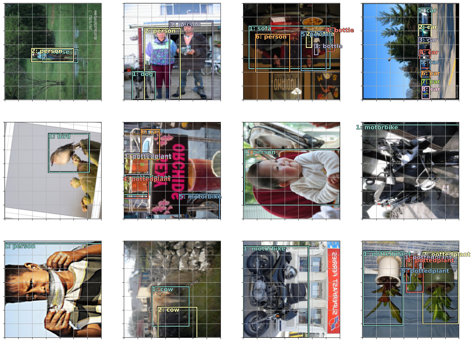

Everything looks fine! We have correct bounding boxes and their corresponding classes

Map to Ground-Truth and Loss function

As you might guess, There are 2 components forming the Object Detection Loss: Classification Loss (For the class) and Localization Loss (For the bounding box)

The idea is, for each image, we will: - Calculate the Intersection-over-Union (IoU) of each predefined Anchor Box with the Object Bounding Box. - Assign the label for each cell (Map to ground truth) according to the IoUs. Background will be assigned to Cell which overlaps with no object - Calculate the Classification Loss for all Cells - Calculate the Bounding Box Location Loss only for Cells responsible to Objects (no Background) - Take the sum of these 2 losses

Note

Currently, we will loop for each image in a batch to calculate its loss and then sum them all. I think we might have a better way to vectorize these operations, or, calculate everything in one shot directly with a batch tensor

def get_y(bbox,clas):
    """
    Remove the zero batching from a batch
    
    Because the number of object in each image are different so
    we need to zero padding for batching 
    """
    bbox = bbox.view(-1,4)
    clas = clas.view(-1,1)
    bb_keep = ((bbox[:,2]-bbox[:,0])>0).nonzero()[:,0]
    return TensorBase(bbox)[bb_keep],TensorBase(clas)[bb_keep]

one_batch[2][idx]

TensorMultiCategory([16, 16, 16, 16, 14,  7,  0,  0,  0,  0,  0,  0,  0,  0,  0,
                      0,  0,  0,  0,  0,  0,  0,  0,  0,  0,  0,  0,  0,  0,  0,
                      0,  0,  0,  0,  0,  0,  0], device='cuda:0')

get_y(one_batch[1][idx], one_batch[2][idx])

(TensorBBox([[ 0.0966, -1.0172,  0.4870, -0.4764],
             [-0.3311, -1.0029,  0.0835, -0.4559],
             [-0.3511, -1.0028,  0.0783, -0.4872],
             [ 0.1286, -1.0201,  0.5700, -0.5041],
             [ 0.4902,  0.1488,  1.0261,  0.9663],
             [-0.8546, -0.6447, -0.2425, -0.2718]], device='cuda:0'),
 TensorBBox([[16],
             [16],
             [16],
             [16],
             [14],
             [ 7]], device='cuda:0'))

We can see that all the zero values are removed before continuing to process

def hw2corners(ctr, hw): 
    # Function to convert BB format: (centers and dims) -> corners
    return torch.cat([ctr-hw/2, ctr+hw/2], dim=1)

The Activations are passed to a Tanh function to rescale their values to -1 -> 1. Then they are processed to make coherent with the Grid Coordinates:

The center of each cell’s prediction stays in the cell
The size of each cell’s prediction can be varied from 1/2 to 3/2 cell’s size to give more flexibility

Tip

The bounding box activations are in [x_center, y_center, width, height] format to easily define the min/max scale to the anchor box

def actn_to_bb(actn, anchors):
    actn_bbs = torch.tanh(actn)
    actn_centers = (actn_bbs[:,:2]/2 * grid_sizes) + anchors[:,:2]
    actn_hw = (actn_bbs[:,2:]/2+1) * anchors[:,2:]
    return hw2corners(actn_centers, actn_hw)

def one_hot_embedding(labels, num_classes):
    return torch.eye(num_classes)[labels].cuda()

def intersect(box_a, box_b):
    """
    Intersect area between to bounding boxes
    """
    max_xy = torch.min(box_a[:, None, 2:], box_b[None, :, 2:])
    min_xy = torch.max(box_a[:, None, :2], box_b[None, :, :2])
    inter = torch.clamp((max_xy - min_xy), min=0)
    return inter[:, :, 0] * inter[:, :, 1]

def box_sz(b): return ((b[:, 2]-b[:, 0]) * (b[:, 3]-b[:, 1]))

def jaccard(box_a, box_b):
    """
    Jaccard or Intersection over Union
    """
    inter = intersect(box_a, box_b)
    union = box_sz(box_a).unsqueeze(1) + box_sz(box_b).unsqueeze(0) - inter
    return inter / union

Map to Ground Truth (Visualization below). The idea is looping through all anchor boxes and calculating the overlaps with the Ground Truth bounding boxes, then assigning each Anchor Box to the corresponding class

def map_to_ground_truth(overlaps):
    prior_overlap, prior_idx = overlaps.max(1) # 3
    gt_overlap, gt_idx = overlaps.max(0) # 16
    gt_overlap[prior_idx] = 1.99
    for i,o in enumerate(prior_idx): gt_idx[o] = i
    return gt_overlap,gt_idx

For calculating loss, we will loop through every images in a batch and calculate loss for each image (ssd_1_loss), then summing the result with ssd_loss. The Classification Loss (loss_f) currently is left empty as we will discussion it later in the next section.

def ssd_1_loss(b_c,b_bb,bbox,clas):
    bbox,clas = get_y(bbox,clas)
    bbox = (bbox+1)/2
    a_ic = actn_to_bb(b_bb, anchors)
    overlaps = jaccard(bbox.data, anchor_cnr.data)
    gt_overlap,gt_idx = map_to_ground_truth(overlaps)
    gt_clas = clas[gt_idx]
    pos = gt_overlap > 0.4
    pos_idx = torch.nonzero(pos)[:,0]
    gt_clas[~pos] = 0  # Assign the background to idx 0
    gt_bbox = bbox[gt_idx]
    loc_loss = ((TensorBase(a_ic[TensorBase(pos_idx)]) - TensorBase(gt_bbox[TensorBase(pos_idx)])).abs()).mean()
    clas_loss  = loss_f(b_c, gt_clas)
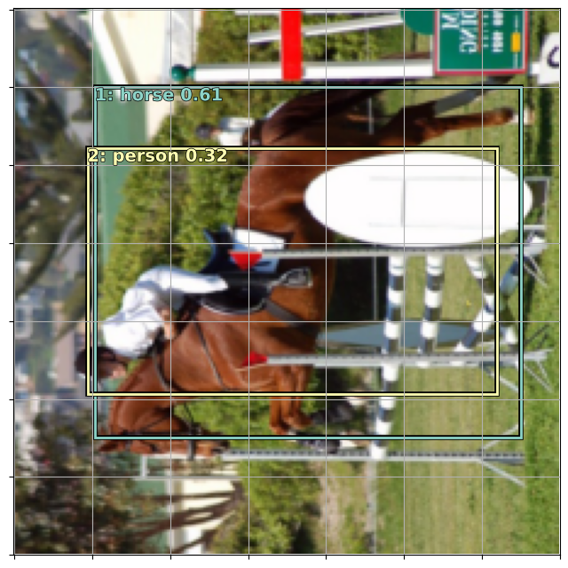
    return loc_loss, clas_loss

anchor_cnr = hw2corners(anchors[:,:2], anchors[:,2:]).cuda()

Showing Map To Ground Truth

As mentioned earlier, Map-to-Ground-Truth is a very important step for calculating loss. We should show it to make sure everything looks fine

idx = 0
bbox = one_batch[1][idx].cuda()
clas = one_batch[2][idx].cuda()

bbox,clas = get_y(bbox,clas)
bbox = (bbox+1)/2
# a_ic = actn_to_bb(b_bb, anchors)
overlaps = jaccard(bbox.data, anchor_cnr.data)
gt_overlap,gt_idx = map_to_ground_truth(overlaps)
gt_clas = clas[gt_idx]
pos = gt_overlap > 0.4
pos_idx = torch.nonzero(pos)[:,0]
gt_clas[~pos] = 0  # Assign the background to idx 0
gt_bbox = bbox[gt_idx]

ima = one_batch[0][idx].permute(2,1,0).cpu()

fig, ax = plt.subplots(figsize=(7,7))
torch_gt(ax, ima, bbox, clas)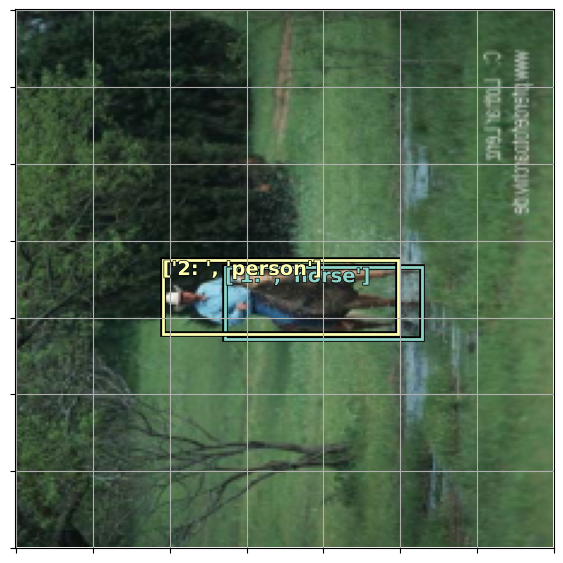

fig, ax = plt.subplots(figsize=(7,7))
torch_gt(ax, ima, anchor_cnr, gt_clas)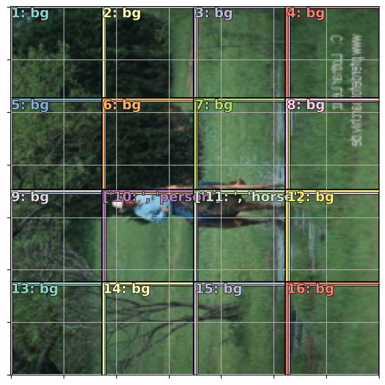

sz = 224

Classificaton Loss: Binary Cross Entropy and why Focal Loss

2 tricks can be used for Classification Loss:

Binary Cross-Entropy Loss without background
Further improve Binary Cross-Entropy Loss with Focal Loss

Binary Cross-Entropy

If we treat the Background Class as one class and ask the Model to understand what is a Background, it might be too difficult. We can translate it to a set of easier questions: Is it a Cat? Is it a Dog? … through all the classes, which is exactly what Binary Cross-Entropy does

Focal Loss

The classification task in object detection is very imbalance that we have a lot of background objects (check the Match to Ground-Truth image above). If we just use Binary Cross-Entropy Loss function, it will try all efforts to improve background classification

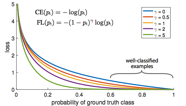
Quote from fastai2018 course:

The blue line is the binary cross entropy loss. If the answer is not a motorbike, and I said “I think it’s not a motorbike and I am 60% sure” with the blue line, the loss is still about 0.5 which is pretty bad. So if we want to get our loss down, then for all these things which are actually back ground, we have to be saying “I am sure that is background”, “I am sure it’s not a motorbike, or a bus, or a person” — because if I don’t say we are sure it is not any of these things, then we still get loss.

That is why the motorbike example did not work. Because even when it gets to lower right corner and it wants to say “I think it’s a motorbike”, there is no payoff for it to say so. If it is wrong, it gets killed. And the vast majority of the time, it is background. Even if it is not background, it is not enough just to say “it’s not background” — you have to say which of the 20 things it is.

So the trick is to trying to find a different loss function that looks more like the purple line. Focal loss is literally just a scaled cross entropy loss. Now if we say “I’m .6 sure it’s not a motorbike” then the loss function will say “good for you! no worries”.

class BCE_Loss(nn.Module):
    def __init__(self, num_classes):
        super().__init__()
        self.num_classes = num_classes

    def forward(self, pred, targ):
        t = one_hot_embedding(targ.squeeze(), self.num_classes)
        t = t[:,1:] # Start from 1 to exclude the Background
        x = pred[:,1:]
        w = self.get_weight(x,t)
        return F.binary_cross_entropy_with_logits(x, t, w.detach(), reduction='sum')/self.num_classes
    
    def get_weight(self,x,t): return None

class FocalLoss(BCE_Loss):
    def get_weight(self,x,t):
        alpha,gamma = 0.25,1
        p = x.sigmoid()
        pt = p*t + (1-p)*(1-t)
        w = alpha*t + (1-alpha)*(1-t)
        return w * (1-pt).pow(gamma)

The ssd_loss will loop through every image in a batch and accumulate loss

def ssd_loss(pred, bbox, clas):
    lcs, lls = 0., 0.
    W = 30
    for b_c, b_bb, bbox, clas in zip(*pred, bbox, clas):
        loc_loss, clas_loss = ssd_1_loss(b_c, b_bb, bbox, clas)
        lls += loc_loss
        lcs += clas_loss
    return lls + lcs

loss_f = FocalLoss(len(dls.vocab))

Training Simple Model

model = nn.Sequential(body, head_reg4)

learner = Learner(dls, model, loss_func=ssd_loss)

learner.fit_one_cycle(5, 1e-3)

epoch	train_loss	valid_loss	time
0	34.889286	28.454723	00:25
1	32.127403	29.533695	00:23
2	30.588394	26.637667	00:23
3	29.455709	25.630453	00:23
4	28.651590	25.509596	00:23

The loss decreases, and the model can learn something. Looking at the results shown below, we can see that the predictions are not so bad but not particularly good either. In the next session, we can see how to improve the results with more anchor boxes

Show Results

one_batch = dls.valid.one_batch()
learner.model.eval();
pred = learner.model(one_batch[0])
b_clas, b_bb = pred
x = one_batch[0]

fig, axes = plt.subplots(3, 4, figsize=(16, 12))
for idx,ax in enumerate(axes.flat):
    ima = x.permute(0,3,2,1).cpu()[idx]
#     ima=md.val_ds.ds.denorm(x)[idx]
    bbox,clas = get_y(y[0][idx], y[1][idx])
    a_ic = actn_to_bb(b_bb[idx], anchors)
    torch_gt(ax, ima, a_ic, b_clas[idx].max(1)[1], b_clas[idx].max(1)[0].sigmoid(), 0.21)
#plt.tight_layout()
plt.subplots_adjust(wspace=0.15, hspace=0.15)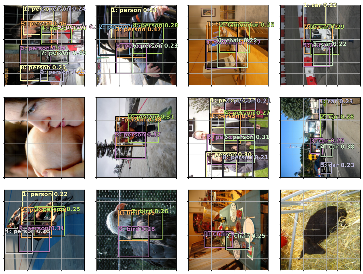

More anchors

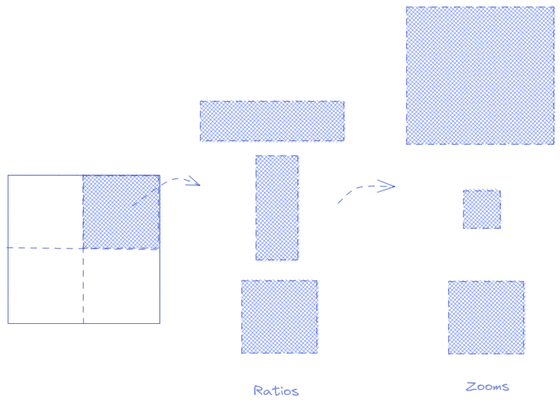
As said earlier, the anchor box is a hint for the model to not go too far and focus on a part of the image. So obviously, 4x4 grid is not enough to predict an object of any size. In this part, by adding more Conv2d layers, we will have 3 grids: 4x4, 2x2, 1x1 and each cell will have 9 variations: 3-zooms and 3-ratios

The total number of anchors is: (16 + 4 + 1) x 9 = 189 anchors

# This is for release the GPU memrory while experimenting. I guess it is not enough. Please tell me if you know a better way
del learner
del model
import gc; gc.collect()
torch.cuda.empty_cache()

anc_grids = [4,2,1]
anc_zooms = [0.7, 1., 1.3]
anc_ratios = [(1.,1.), (1.,0.5), (0.5,1.)]
anchor_scales = [(anz*i,anz*j) for anz in anc_zooms for (i,j) in anc_ratios]
k = len(anchor_scales)
anc_offsets = [1/(o*2) for o in anc_grids]
k

anc_x = np.concatenate([np.repeat(np.linspace(ao, 1-ao, ag), ag)
                        for ao,ag in zip(anc_offsets,anc_grids)])
anc_y = np.concatenate([np.tile(np.linspace(ao, 1-ao, ag), ag)
                        for ao,ag in zip(anc_offsets,anc_grids)])
anc_ctrs = np.repeat(np.stack([anc_x,anc_y], axis=1), k, axis=0)

anc_x

array([0.125, 0.125, 0.125, 0.125, 0.375, 0.375, 0.375, 0.375, 0.625,
       0.625, 0.625, 0.625, 0.875, 0.875, 0.875, 0.875, 0.25 , 0.25 ,
       0.75 , 0.75 , 0.5  ])

anc_sizes  =   np.concatenate([np.array([[o/ag,p/ag] for i in range(ag*ag) for o,p in anchor_scales])
               for ag in anc_grids])
grid_sizes = torch.tensor(np.concatenate([np.array([ 1/ag       for i in range(ag*ag) for o,p in anchor_scales])
               for ag in anc_grids]), requires_grad=False).unsqueeze(1).cuda()
anchors = torch.tensor(np.concatenate([anc_ctrs, anc_sizes], axis=1), requires_grad=False).float().cuda()
anchor_cnr = hw2corners(anchors[:,:2], anchors[:,2:]).cuda()

anchor_cnr.shape

torch.Size([189, 4])

We need to adjust the SSD head a little bit. We will add more Conv2D layer with StdConv (to create 2x2 and 1x1 grids). After each StdConv is an OutConv to handle the Classification prediction and Localization prediction

class SSD_MultiHead(nn.Module):
    def __init__(self, k, bias):
        super().__init__()
        self.drop = nn.Dropout(drop)
        self.sconv0 = StdConv(512,256, stride=1, drop=drop)
        self.sconv1 = StdConv(256,256, drop=drop)
        self.sconv2 = StdConv(256,256, drop=drop)
        self.sconv3 = StdConv(256,256, drop=drop)
        self.out0 = OutConv(k, 256, bias)
        self.out1 = OutConv(k, 256, bias)
        self.out2 = OutConv(k, 256, bias)
        self.out3 = OutConv(k, 256, bias)

    def forward(self, x):
        x = self.drop(F.relu(x))
        x = self.sconv0(x)
        x = self.sconv1(x)
        o1c,o1l = self.out1(x)
        x = self.sconv2(x)
        o2c,o2l = self.out2(x)
        x = self.sconv3(x)
        o3c,o3l = self.out3(x)
        return [torch.cat([o1c,o2c,o3c], dim=1),
                torch.cat([o1l,o2l,o3l], dim=1)]

drop=0.4

head_reg4 = SSD_MultiHead(k, -4.)

body = create_body(resnet34(True))
model = nn.Sequential(body, head_reg4)

learner = Learner(dls, model, loss_func=ssd_loss)

# learner.lr_find()

learner.fit_one_cycle(20, 1e-3)

epoch	train_loss	valid_loss	time
0	79.482658	65.257332	00:24
1	77.919846	64.182114	00:24
2	75.337402	69.358673	00:24
3	70.927734	73.576935	00:24
4	65.866829	58.502281	00:24
5	61.796001	51.171406	00:24
6	58.571583	47.785007	00:24
7	55.809723	45.772766	00:24
8	53.606243	45.726265	00:25
9	51.751816	45.473743	00:24
10	49.946224	43.707134	00:24
11	48.457012	42.950340	00:25
12	46.938705	40.909351	00:24
13	45.661766	40.690815	00:24
14	44.419174	40.372437	00:25
15	43.232628	39.393692	00:24
16	42.119759	38.884872	00:24
17	41.290310	38.704178	00:24
18	40.546024	38.666664	00:24
19	39.970467	38.707432	00:24

Show results

one_batch = dls.valid.one_batch()
learner.model.eval();
pred = learner.model(one_batch[0])
b_clas, b_bb = pred
x = one_batch[0]

fig, axes = plt.subplots(3, 4, figsize=(16, 12))
for idx,ax in enumerate(axes.flat):
    ima = x.permute(0,3,2,1).cpu()[idx]
#     ima=md.val_ds.ds.denorm(x)[idx]
    bbox,clas = get_y(y[0][idx], y[1][idx])
    a_ic = actn_to_bb(b_bb[idx], anchors)
    torch_gt(ax, ima, a_ic, b_clas[idx].max(1)[1], b_clas[idx].max(1)[0].sigmoid(), thresh=0.21)
#plt.tight_layout()
plt.subplots_adjust(wspace=0.15, hspace=0.15)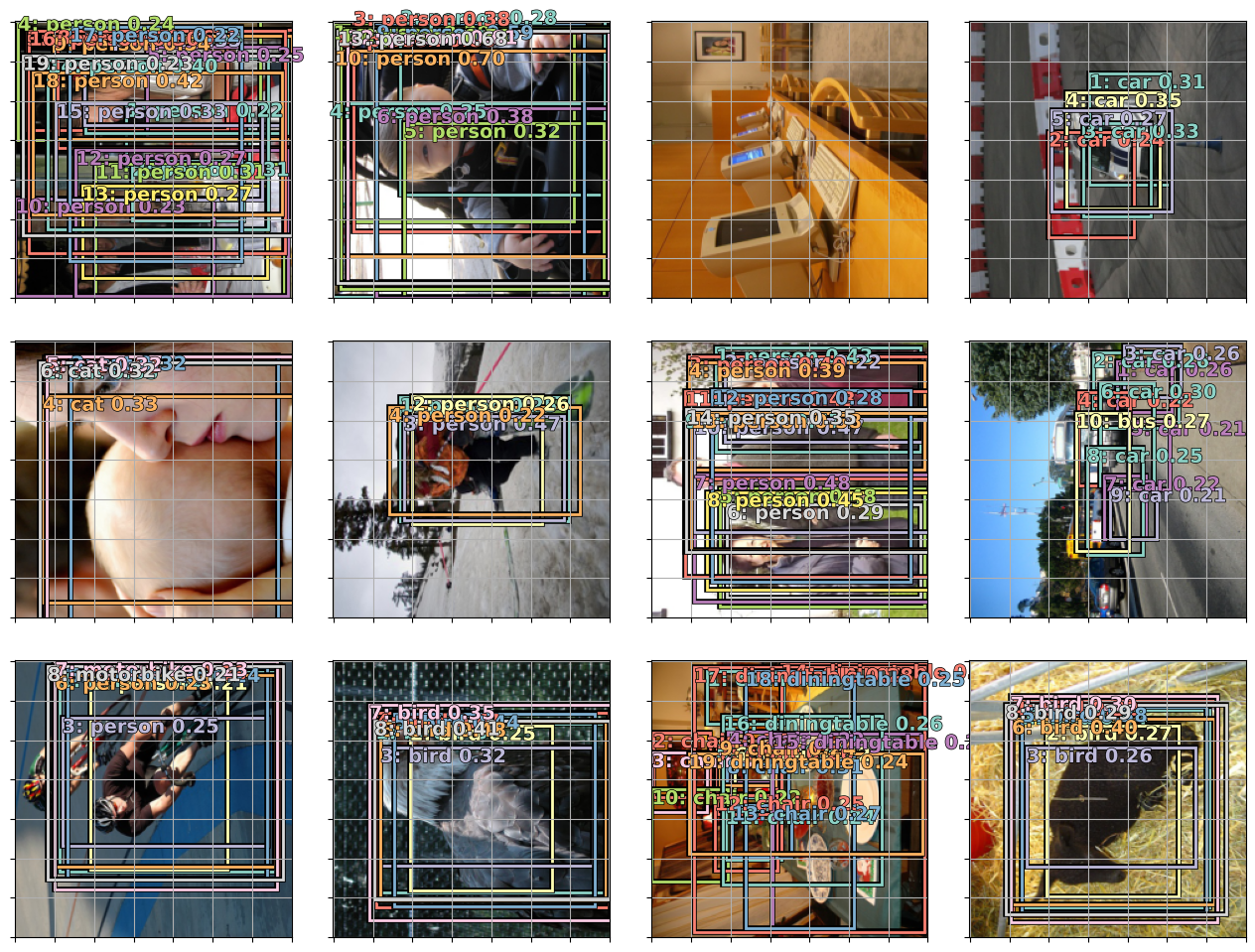

The result looks better than the simple version above

Non Maximum Suppression (NMS)

You can see in the previous results, that having a lot of Anchor Boxes leads to many overlaps. You can use Non Maximum Suppression, a technique to choose one bounding box out of many overlapping ones

def nms(boxes, scores, overlap=0.5, top_k=100):
    keep = scores.new(scores.size(0)).zero_().long()
    if boxes.numel() == 0: return keep
    x1 = boxes[:, 0]
    y1 = boxes[:, 1]
    x2 = boxes[:, 2]
    y2 = boxes[:, 3]
    area = torch.mul(x2 - x1, y2 - y1)
    v, idx = scores.sort(0)  # sort in ascending order
    idx = idx[-top_k:]  # indices of the top-k largest vals
    xx1 = boxes.new()
    yy1 = boxes.new()
    xx2 = boxes.new()
    yy2 = boxes.new()
    w = boxes.new()
    h = boxes.new()

    count = 0
    while idx.numel() > 0:
        i = idx[-1]  # index of current largest val
        keep[count] = i
        count += 1
        if idx.size(0) == 1: break
        idx = idx[:-1]  # remove kept element from view
        # load bboxes of next highest vals
        torch.index_select(x1, 0, idx, out=xx1)
        torch.index_select(y1, 0, idx, out=yy1)
        torch.index_select(x2, 0, idx, out=xx2)
        torch.index_select(y2, 0, idx, out=yy2)
        # store element-wise max with next highest score
        xx1 = torch.clamp(xx1, min=x1[i])
        yy1 = torch.clamp(yy1, min=y1[i])
        xx2 = torch.clamp(xx2, max=x2[i])
        yy2 = torch.clamp(yy2, max=y2[i])
        w.resize_as_(xx2)
        h.resize_as_(yy2)
        w = xx2 - xx1
        h = yy2 - yy1
        # check sizes of xx1 and xx2.. after each iteration
        w = torch.clamp(w, min=0.0)
        h = torch.clamp(h, min=0.0)
        inter = w*h
        # IoU = i / (area(a) + area(b) - i)
        rem_areas = torch.index_select(area, 0, idx)  # load remaining areas)
        union = (rem_areas - inter) + area[i]
        IoU = inter/union  # store result in iou
        # keep only elements with an IoU <= overlap
        idx = idx[IoU.le(overlap)]
    return keep, count

def show_nmf(idx):
    ima = one_batch[0][idx].permute(2,1,0).cpu()
    bbox = one_batch[1][idx].cuda()
    clas = one_batch[2][idx].cuda()
    bbox,clas = get_y(bbox,clas)
    
    a_ic = actn_to_bb(b_bb[idx], anchors)
    clas_pr, clas_ids = b_clas[idx].max(1)
    clas_pr = clas_pr.sigmoid()

    conf_scores = b_clas[idx].sigmoid().t().data

    out1,out2,cc = [],[],[]
    for cl in range(1, len(conf_scores)):
        c_mask = conf_scores[cl] > 0.25
        if c_mask.sum() == 0: continue
        scores = conf_scores[cl][c_mask]
        l_mask = c_mask.unsqueeze(1).expand_as(a_ic)
        boxes = a_ic[l_mask].view(-1, 4)
        ids, count = nms(boxes.data, scores, 0.4, 50)
        ids = ids[:count]
        out1.append(scores[ids])
        out2.append(boxes.data[ids])
        cc.append([cl]*count)
    if not cc:
        print(f"{i}: empty array")
        return
    cc = torch.tensor(np.concatenate(cc))
    out1 = torch.cat(out1)
    out2 = torch.cat(out2)

    fig, ax = plt.subplots(figsize=(8,8))
    torch_gt(ax, ima, out2, cc, out1, 0.1)

for i in range(25, 35): show_nmf(i)

25: empty array
28: empty array
31: empty array
32: empty array